Fama French and Multi-Factor Models of Risk

Lucas S. Macoris (FGV-EAESP)

Outline

• This lecture is mainly based the following textbooks:
  1. Tidy Finance (Scheuch, Voigt, and Weiss 2023)
  2. R for Data Science (Wickham, Mine Cetinkaya-Rundel, and Grolemund 2023)

Coding Replications

For coding replications, whenever applicable, please follow this page or hover on the specific slides with containing coding chunks.

1. Ensure that you have your session properly set-up according to the instructions outlined in the course webpage
2. In the webpage, you can also find a detailed discussion of the examples covered in this lecture

Disclaimer

Disclaimer

The information presented in this lecture is for educational and informational purposes only and should not be construed as investment advice. Nothing discussed constitutes a recommendation to buy, sell, or hold any financial instrument or security. Investment decisions should be made based on individual research and consultation with a qualified financial professional. The presenter assumes no responsibility for any financial decisions made based on this content.

All code used in this lecture is publicly available and is also shared on my GitHub page. Participants are encouraged to review, modify, and use the code for their own learning and research purposes. However, no guarantees are made regarding the accuracy, completeness, or suitability of the code for any specific application.

For any questions or concerns, please feel free to reach out via email at lucas.macoris@fgv.br

What if \(\alpha\) is consistently different from zero?

• Let’s go back to our \(\alpha\) definition for a given stock \(i\):

\[ \alpha_i = E[R_i] - R_i \]

• As we discussed, if you assume that CAPM is the correct model to explain expected returns, competition in financial markets should make \(\alpha \rightarrow 0\) in equilibrium:

  1. Stocks above the SML are cheap, so the prices should rise (positive alpha).
  2. Stocks below the SML are expensive, so the prices should drop (negative alpha).

• However, over the years since the discovery of the CAPM, it has become increasingly clear that forming portfolios based on market capitalization, book-to-market ratios, and past returns, investors can construct trading strategies that have a \(\small alpha>0\)

• Why? There can be two reasons why positive-alpha strategies exist in a persistent way

Why \(\alpha\) is consistently different from zero?

Reason #1: Investors are systematically ignoring positive-NPV investment opportunities:

• The CAPM correctly computes required risk premiums, but investors are ignoring opportunities to earn extra returns without bearing any extra risk
• That could happen either because they are unaware of them or because the costs to implement the strategies are larger than the NPV of undertaking them

\(\rightarrow\) This explanation goes straight to the hypotheses outlined by the CAPM!

• The only way a positive-NPV opportunity can persist in a market is if some barrier to entry restricts competition. Nowadays, this hypothesis seems unlikely:

  1. Information required to form the portfolios is readily available;
  2. Trading costs are decreasing

Why \(\alpha\) is consistently different from zero? Continued

Reason #2: The positive-alpha trading strategies contain risk that investors are unwilling to bear but the CAPM does not capture:

1. A stock’s beta with the market portfolio does not adequately measure a stock’s systematic risk

2. Because of that, the CAPM does not correctly compute the risk premium as it leaves out important risk factors that investors care about other than the market sensitivity!

• In other words, the positive alphas from the trading strategy are really returns for bearing risk that investors are averse to but the model does not capture:

1. We assumed that investor would always seek for the best risk \(\times\) return combination

2. However, investors may stick with inefficient portfolios because they care about risk characteristics other than the volatility of their traded portfolio. For instance, they prefer to not be exposed to the sector they work in or to specific industries (i.e., ESG-based decisions)

Moving Beyond the CAPM

• We previously defined that the required return for any given security \(i\) should follow:

\[ E[R_i] = R_f + \beta_i^P \times (E[R_P - R_f]) \]

1. At first, we were agnostic on what \(P\), the portfolio returns, should stand for
2. When we introduced the CAPM, we claimed that \(P=M\) - i.e, the efficient portfolio is the market portfolio

• However, real-world frictions points us to an uncomfortable outcome:

  1. The CAPM assumes a single risk factor (market risk), but…
  2. There is empirical evidence that shows additional factors can explain anomalies

\(\rightarrow\) When the market portfolio is not efficient, we have to find a method to identify an efficient portfolio before we can use the above equation!

Size Effect

• Idea: small market capitalization stocks have historically earned higher average returns than the market portfolio, even after accounting for their higher betas

• A way to replicate this thesis is to split stocks each year into 10 portfolios by ranking them based on their market capitalizations:

  1. The first portfolio had the 10% smallest stocks in terms of market capitalization
  2. The second portfolio had the 20% smallest stocks; and so on, until…
  3. The tenth portfolio had the 10% biggest stocks in terms of market capitalization

Calculating the monthly excess returns and the beta of each decile portfolio, we see that:

1. Portfolios with higher betas yield higher future returns (as expected)
2. Most portfolios were above the security market (\(\small \alpha>0\))
3. The smallest deciles - i.e, small-cap firms - exhibit the most extreme effect

Book-to-Market Ratio

• As with Size, a similar rationale could be applied to stocks that have higher levels of Market Value of Equity vis-a-vis their historical values (Book Value of Equity)

• Idea: small market capitalization stocks have historically earned higher average returns than the market portfolio, even after accounting for their higher betas

  1. High book-to-market stocks have historically earned higher average returns than low book-to-market stocks
  2. Stocks with high book-to-market ratios are value stocks, and those with low book-to-market ratios are growth stocks

Calculating the monthly excess returns and the beta of each decile portfolio, we see that:

1. In this case, value stocks - i.e, the stocks in the highest deciles - tend to present higher \(\alpha\)
2. As such, a strategy that goes long on value stocks and short on growth stocks tends to present positive \(\alpha\)

Multifactor Models of Risk

• When we first introduced the CAPM, we implicitly assumed that there was a single portfolio (or “factor”) that represented the efficient portfolio: the market (a “single factor” portfolio)

• However, it is not actually necessary to identify the efficient portfolio itself, as long as you identify a collection of portfolios from which the efficient portfolio can be constructed

• A Multi-Factor Model is a pricing model that uses more than one portfolio (“factors”) to approximate the efficient portfolio:

\[ \small E[R_i] = R_f + \beta_i^{\text{F1}} \times \underbrace{(E[R_{\text{F1}} - R_f])}_{\text{Excess return for Factor 1}}+ \beta_i^{\text{F2}} \times \underbrace{(E[R_{\text{F2}} - R_f])}_{\text{Excess return for Factor 2}}+...+\beta_i^{\text{Fn}} \times \underbrace{(E[R_{\text{Fn}} - R_f])}_{\text{Excess return for Factor n}} \]

• Each \(\beta_i^{n}\) here is called a factor beta: like the CAPM, it is the expected % change in the excess return of a security for a 1% change in the excess return of that factor portfolio, holding everything else constant

Multifactor Models of Risk, continued

• The previous equation showed that that we can write the risk premium of any marketable security as the sum of the risk premium of each factor multiplied by the sensitivity of the stock with that factor:

  1. Single-factor: We use an presumably efficient portfolio, it will alone capture all systematic risk (for example, the CAPM)
  2. Multifactor: If we use multiple portfolios as factors, then together these factors will capture all systematic risk - this is also known as the Arbitrage Pricing Theory (APT)

• Multifactor models allow investors to break the risk premium down into different factors:

  1. As they might not be equally averse to the different factors, multifactor models allows investors to tailor their risk exposure
  2. This idea of tailoring risk exposures based on common risk factors has become increasingly known amongst practitioners as a smart beta strategy - click here for an extensive list of factor ETFs from Fidelity

Which factors (portfolios) to use?

• If investors can tailor their risk exposure to specific risk factors, then the next question is: which risk factors an investor should be exposed to?

• Some important risk factors found in the previous literature include, but not limited to:

  1. Market Strategy: the most straightforward example is to expose to the market itself, like the CAPM did. Even if the market portfolio is not efficient, it still captures many components of systematic risk

  2. Market Capitalization Strategy: a trading strategy that each year buys portfolio S (small stocks) and finances this position by short selling portfolio B (big stocks) has produced positive risk-adjusted returns historically. This is called a small-minus-big (SMB) portfolio

  3. Book-to-Market Strategy: a trading strategy that each year buys a portfolio of growth stocks and finances it by selling value stocks. This is called a high-minus-low (HML) portfolio

Example: the Fama-French model

• A direct application of the previous slide is the Fama-French portfolio (Fama and French 1993), which considers the Market, the Market Capitalization Strategy (Size), and the Book-to-Market (Value) strategy:

\[\small E[R_i] = R_f + \beta_s^m \times \underbrace{(E[R_m]− R_f)}_{\text{Market}} + \beta_s^{SMB} \times \underbrace{E[R_{SMB}]}_{\text{Size}} + \beta_s^{HML} \times \underbrace{E[R_{HML}]}_{\text{Market Cap.}}\]

1. Note that we can price the required returns for a given security \(i\) according to its exposure (the \(\beta\)’s) to each of the factor portfolios
2. Before, we claimed using the CAPM that only the first factor should drive required returns (i.e., the market)
3. If investors also care about other risk factors, the exposure of a given security needs to take that into account when estimating the required returns!

Application: Hedge Fund Performance Evaluation

• One of the most widely known examples of applications using the Fama-French model is to assess a hedge fund’s true skill in generating excess returns:
  1. Many hedge-fund managers claim to generate excess returns (\(\alpha\))…
  2. …but after adjusting for Fama-French factors, true skill is revealed!
• Investors can use this model to determine whether returns come from skill (true alpha) or simply exposure to common risk factors
  1. If a fund shows positive \(\alpha\) after accounting for the Fama-French factors, it suggests manager skill
  2. If returns are fully explained by factors, performance comes from risk exposure, not manager’s skill
• Furthermore, investors can understand how exposed a given strategy is to the most common risk factors, and understand the determinants of the fund’s returns over time

Hands-On Exercise

• You work as a quantitative analyst at Axe Capital. You have been given the task of analyzing a couple of Hedge Fund strategies and assess whether they have generated true excess returns that could have been attributed to their manager’s skill:

  1. What is the historical performance of each strategy over time?
  2. Which strategies, according to the CAPM model, have generated \(\alpha>0\)?
  3. Which strategies, according to the Fama-French model, have generated \(\alpha>0\)?

Specific Instructions

1. You will be using some of the data contained in the edhec dataset - click here for a detailed explanation on the dataset.
2. Model estimation should be done at the monthly level

About the dataset

• The edhec dataset, from the EDHEC Risk and Asset Management Research Center, is a dataset that covers monthly Hedge Fund returns starting from 1997

• Each series of returns represents a Hedge Fund strategy that seeks to exploit a given type of market anomaly:

  1. Convertible Arbitrage - click here for details
  2. Event Driven - click here for details
  3. Merger Arbitrage - click here for details
  4. Relative Value - click here for details
  5. Distressed Securities - click here for details
  6. CTA Global - click here for details

Step 1: Loading the data

• The first step is to load the data on historical returns on hedge fund strategies. For that, the edhec dataset - provided in the PerformanceAnalytics package, contains the historical monthly returns for a handful of alternative global strategies

• I have already prepped the data for you in an .rds file that can be downloaded using the Download Data button below or directly through eClass®. An .rds file is an R object that can be loaded directly into your R session

• To load an .rds file, you can either double-click and open using RStudio, or run the following command:

#Assuming that the file is in the correct folder
hf_data=readRDS('hf_data.rds')

• Note that the object that has been loaded is an xts object, which inherits several useful properties for working with time series data!

Step 2: Historical Performance

• It is very easy to work with time series using the base R capabilities. For example, you can pass call cumprod(1+x) in your dataset, and R understands that you want to do these operations column-wise

• Alternatively, you can use the steps from the previous lectures to get the data into a proper format for using ggplot2

• Code
• Output

#Apply the cumprod function to all columns
cumprod(1+hf_data)-1%>%head()

           Convertible.Arbitrage CTA.Global Distressed.Securities
1997-01-01            0.01190000 0.03930000            0.01780000
1997-02-01            0.02434637 0.07027114            0.03021716
1997-03-01            0.03233627 0.06802357            0.02898090
1997-04-01            0.04121436 0.04986717            0.03206784
1997-05-01            0.05745731 0.04829237            0.05611502
1997-06-01            0.07987540 0.05720285            0.07903272
1997-07-01            0.10071700 0.11968354            0.10428208
1997-08-01            0.11546661 0.06672251            0.12051503
1997-09-01            0.12907530 0.08784362            0.15973306
1997-10-01            0.14036605 0.07718275            0.15231077
       ...                                                       
2020-08-01            3.68582245 1.94567988            4.80813414
2020-09-01            3.71065731 1.88941739            4.84821027
2020-10-01            3.74127659 1.87872655            4.83300492
2020-11-01            3.87972186 1.91471063            5.08149093
2020-12-01            3.98561183 2.04645555            5.26819270
2021-01-01            4.10875644 2.03670689            5.41800251
2021-02-01            4.20531194 2.13236316            5.62081139
2021-03-01            4.18032644 2.14645879            5.72873061
2021-04-01            4.17980841 2.22512026            5.87407120
2021-05-01            4.20881533 2.27801223            5.98955559
           Emerging.Markets Equity.Market.Neutral Event.Driven
1997-01-01        0.0791000            0.01890000   0.02130000
1997-02-01        0.1357527            0.02919089   0.02987892
1997-03-01        0.1221237            0.03083760   0.02751020
1997-04-01        0.1354770            0.04310456   0.02699644
1997-05-01        0.1712445            0.06281924   0.06253052
1997-06-01        0.2392938            0.08035576   0.08994381
1997-07-01        0.3086943            0.10704054   0.12340508
1997-08-01        0.3000569            0.10892251   0.13138126
1997-09-01        0.3298282            0.13132275   0.16860370
1997-10-01        0.2537620            0.14207031   0.17573218
       ...                                                    
2020-08-01        4.2056980            2.33237019   4.34054821
2020-09-01        4.1296948            2.32570545   4.34161632
2020-10-01        4.1163576            2.31073977   4.35443620
2020-11-01        4.4069667            2.32166521   4.71104165
2020-12-01        4.6524430            2.37149019   4.96860963
2021-01-01        4.7683181            2.37250164   5.06888227
2021-02-01        4.8617648            2.41937941   5.29464469
2021-03-01        4.8142846            2.45425708   5.39535901
2021-04-01        4.9637117            2.50503466   5.57187092
2021-05-01        5.0883532            2.51730228   5.65401930

Step 2: Historical Performance

• Code
• Output

(cumprod(1+hf_data)-1)%>%
  as.data.frame()%>%
  rownames_to_column('date')%>%
  mutate(date=as.Date(date))%>%
  pivot_longer(names_to='strategy',values_to = 'cum_return',cols=2:6)%>%
  ggplot(aes(x=date,y=cum_return,group=strategy,col=strategy))+
  geom_line()+
  scale_x_date(date_breaks = 'years',date_labels='%Y')+
  scale_y_continuous(labels = percent)+
  labs(title='Comparison of hedge fund global strategies over time',
       subtitle='Considering EDHEC dataset of monthly hedge fund returns.',
       col='Strategy',
       x='',
       y='Cumulative Return')+
  theme_minimal()+
  theme(legend.position = 'bottom',
        axis.text.x = element_text(angle=90),
        axis.title = element_text(face='bold',size=12),
        plot.title = element_text(face='bold',size=15),
        plot.subtitle  = element_text(size=12))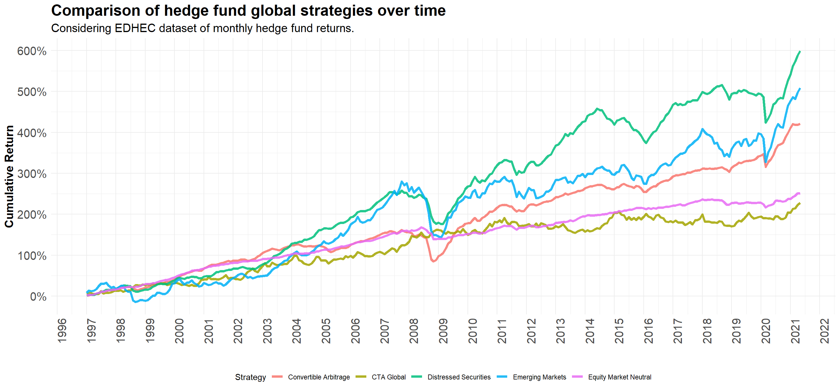

Step 3: Analyzing performance determinants

• Assessing the performance of a given strategy \(i\) can be done by estimating:

\[ R_{i,t}=\alpha + \sum\beta_z R_{z,t}+\varepsilon_{i,t} \] where:

1. \(R_{i,t}\) is the return of a given manager \(i\) in month \(t\)
2. \(R_{i,t}\) is the return of a given factor portfolio \(z\) in month \(t\)

• An OLS regression as described above yields two important components:
  1. The estimated \(\beta_z\)’s are the factor returns, and represent exposure of \(i\) to a given risk factor
  2. The estimated \(\alpha\) is the return that could not be attributed to any other risk factor, and it is thus understood as the manager’s true skill return

Step 3: Analyzing performance determinants, continued

• Our hf_data contains information regarding all Hedge Fund Returns. Where to find information regarding factor portfolio returns?

  1. Luckily, you don’t need to manually create them - there are a couple ways by which you can download historical data on factor portfolio returns
  2. In Kenneth French’s website, you will find historical factor portfolio returns for a variety of economies including the U.S., Developed Economies, Emerging Markets, and Global
  3. In special, we will using monthly factor portfolio returns regarding the three-factor model as in (Fama and French 1993), which you can download below or direclty through eClass®

Step 3: Analyzing performance determinants, continued

• We will now manipulate the data in order to merge both hf_data and the ff3_data

• Code
• Output

#Convert the hf_data to a data.frame object and adjust columns
 hf_data = hf_data%>%
  as.data.frame()%>%
  rownames_to_column('date')%>%
  mutate(date=as.Date(date))

#Merge both datasets by date
merged_df <- hf_data%>%
  #Merge
  left_join(ff3_data, by = "date")%>%
  #Pivot the data for each strategy
  pivot_longer(cols = -c(date, MKT_MINUS_RF, SMB, HML, RF), names_to = "strategy", values_to = "return") %>%
  mutate(excess_return = return - RF)

# A tibble: 1,908 × 8
   date       MKT_MINUS_RF     SMB     HML     RF strategy  return excess_return
   <date>            <dbl>   <dbl>   <dbl>  <dbl> <chr>      <dbl>         <dbl>
 1 1997-01-01       0.0499 -0.0195 -0.0142 0.0045 Converti… 0.0119        0.0074
 2 1997-01-01       0.0499 -0.0195 -0.0142 0.0045 CTA Glob… 0.0393        0.0348
 3 1997-01-01       0.0499 -0.0195 -0.0142 0.0045 Distress… 0.0178        0.0133
 4 1997-01-01       0.0499 -0.0195 -0.0142 0.0045 Emerging… 0.0791        0.0746
 5 1997-01-01       0.0499 -0.0195 -0.0142 0.0045 Equity M… 0.0189        0.0144
 6 1997-01-01       0.0499 -0.0195 -0.0142 0.0045 Event Dr… 0.0213        0.0168
 7 1997-02-01      -0.0049 -0.0322  0.0567 0.0039 Converti… 0.0123        0.0084
 8 1997-02-01      -0.0049 -0.0322  0.0567 0.0039 CTA Glob… 0.0298        0.0259
 9 1997-02-01      -0.0049 -0.0322  0.0567 0.0039 Distress… 0.0122        0.0083
10 1997-02-01      -0.0049 -0.0322  0.0567 0.0039 Emerging… 0.0525        0.0486
# ℹ 1,898 more rows

Step 3: The Fama-French Model

• We can now extend the same rationale to adopt the Fama-French three-factor model, which considers the Market, the Market Capitalization Strategy (Size), and the Book-to-Market (Value) strategy:

\[ \small E[R_i] = R_f + \beta_s^m \times \underbrace{(E[R_m]− R_f)}_{\text{Market}} + \beta_s^{SMB} \times \underbrace{E[R_{SMB}]}_{\text{Size}} + \beta_s^{HML} \times \underbrace{E[R_{HML}]}_{\text{Book-to-Market}} \]

• As before, we will start analyzing the output for one individual strategy individually and then apply the same rationale to replicate the result across all strategies

Step 4: The Fama-French model, one strategy output

• Code
• Output

strategy_name = 'Convertible Arbitrage'
#Get the filtered data
filtered_data = merged_df%>%filter(strategy==strategy_name)
#Estimate the Model
model=lm(excess_return ~ MKT_MINUS_RF + HML + SMB, data = filtered_data)
#Visualize
summary(model)

Call:
lm(formula = excess_return ~ MKT_MINUS_RF + HML + SMB, data = filtered_data)

Residuals:
      Min        1Q    Median        3Q       Max 
-0.115871 -0.004508  0.001188  0.006993  0.053934 

Coefficients:
              Estimate Std. Error t value Pr(>|t|)    
(Intercept)  0.0028446  0.0009793   2.905  0.00394 ** 
MKT_MINUS_RF 0.0601943  0.0139721   4.308  2.2e-05 ***
HML          0.0248444  0.0181225   1.371  0.17138    
SMB          0.0203995  0.0236709   0.862  0.38946    
---
Signif. codes:  0 '***' 0.001 '**' 0.01 '*' 0.05 '.' 0.1 ' ' 1

Residual standard error: 0.01712 on 314 degrees of freedom
Multiple R-squared:  0.06444,   Adjusted R-squared:  0.0555 
F-statistic: 7.209 on 3 and 314 DF,  p-value: 0.000108

Step 4: The Fama-French model, all strategies

• For-loop
• Functional Programming
• Output

#Initially an empy data frame
FF_results = data.frame()
#Get all possible strategies
strategy_names = names(hf_data)[2:7]

#For each i in strategy names:
for(i in strategy_names){
  #Get the filtered data
  filtered_data = merged_df%>%filter(strategy==i)
  #Estimate the Model
  model=lm(excess_return ~ MKT_MINUS_RF + HML + SMB, data = filtered_data)
  #Extract Coefficients applying the tidy() function
  model_tidy=model%>%tidy()%>%mutate(strategy=i)
  #Append
  FF_results=FF_results%>%rbind(model_tidy)
}

FF_results <- merged_df%>%
  #Group by strategy
  group_by(strategy)%>%
  #Nest the data
  nest()%>%
  #For each nest, map the lm() function and the tidy function
  mutate(model = map(data, ~ lm(excess_return ~ MKT_MINUS_RF + HML + SMB, data = .)),
         results = map(model, tidy)) %>%
  #Unnest the results
  unnest(results)%>%
  #Select the desired columns
  select(strategy, term, estimate, std.error, p.value)

# A tibble: 24 × 5
# Groups:   strategy [6]
   strategy              term         estimate std.error  p.value
   <chr>                 <chr>           <dbl>     <dbl>    <dbl>
 1 Convertible Arbitrage (Intercept)   0.00284  0.000979 3.94e- 3
 2 Convertible Arbitrage MKT_MINUS_RF  0.0602   0.0140   2.20e- 5
 3 Convertible Arbitrage HML           0.0248   0.0181   1.71e- 1
 4 Convertible Arbitrage SMB           0.0204   0.0237   3.89e- 1
 5 CTA Global            (Intercept)   0.00274  0.00134  4.13e- 2
 6 CTA Global            MKT_MINUS_RF  0.0326   0.0191   8.88e- 2
 7 CTA Global            HML          -0.00785  0.0248   7.52e- 1
 8 CTA Global            SMB          -0.0503   0.0324   1.21e- 1
 9 Distressed Securities (Intercept)   0.00337  0.00106  1.65e- 3
10 Distressed Securities MKT_MINUS_RF  0.0993   0.0151   2.31e-10
# ℹ 14 more rows

Step 4: which strategies generate positive alpha?

• Code
• Output

FF_results %>%
  filter(term=='(Intercept)')%>%
  mutate(stat_sig=ifelse(p.value<0.01,'Statistically sig. at 1%','Not statistically sig. at 10%'))%>%
  ggplot(aes(x=reorder(strategy,desc(estimate)),y=estimate,fill=stat_sig))+
  geom_col(size=3)+
  geom_text(aes(label = percent(estimate,accuracy=0.01),vjust=-1))+
  #Annotations
  labs(title='Which strategies did generate positive and statistically significant alphas?',
       subtitle = 'Using the Fama-French three-factor model with monthly return data.',
       x = 'Strategy',
       y = 'Alpha (%)',
       fill = 'Stat. Sig')+
  #Scales
  scale_y_continuous(labels = percent)+
  #Custom theme minimal
  theme_minimal()+
  #Adding further customizations
  theme(legend.position='bottom',
        axis.title = element_text(face='bold',size=15),
        axis.text = element_text(size=10),
        plot.title = element_text(size=20,face='bold'),
        plot.subtitle  = element_text(size=15))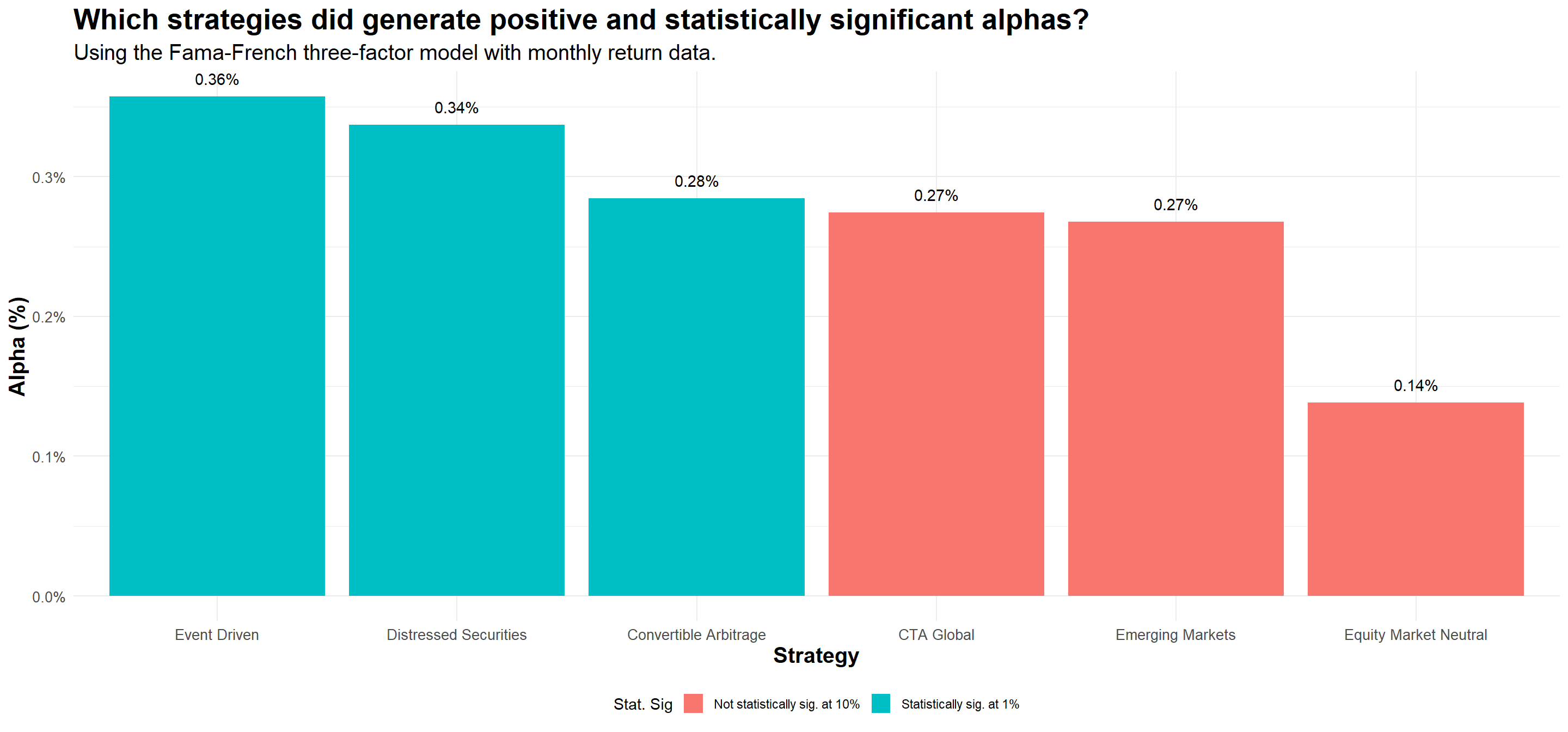

Step 5: The Fama-French Model Attribution

• Code
• Output

FF_results %>%
  filter(term != "(Intercept)")%>%
  group_by(strategy)%>%
  ggplot(aes(x = reorder(term,desc(estimate)), y = estimate, fill = term)) +
  geom_col(position = position_dodge())+
  geom_label(aes(label = round(estimate,2)),position=position_stack(vjust=0.25),col='black',fill='white')+
  theme_minimal()+
  facet_wrap(strategy~.,ncol=3,nrow=2)+
  #Annotations
  labs(title = "Fama-French Factor Loadings by Hedge Fund Strategy",
       x = "Hedge Fund Strategy",
       y = "Factor Loading",
       fill = 'Risk Factor')+
  #Scales+
  scale_fill_manual(values=c('darkred','darkgreen','black'),
                    labels=c('High-minus-Low','Market Excess','Small-minus-Big'))+
  #Custom theme minimal
  theme_minimal()+
  #Adding further customizations
  theme(legend.position='bottom',
        axis.title = element_text(face='bold',size=15),
        axis.text = element_blank(),
        plot.title = element_text(size=20,face='bold'),
        plot.subtitle  = element_text(size=15))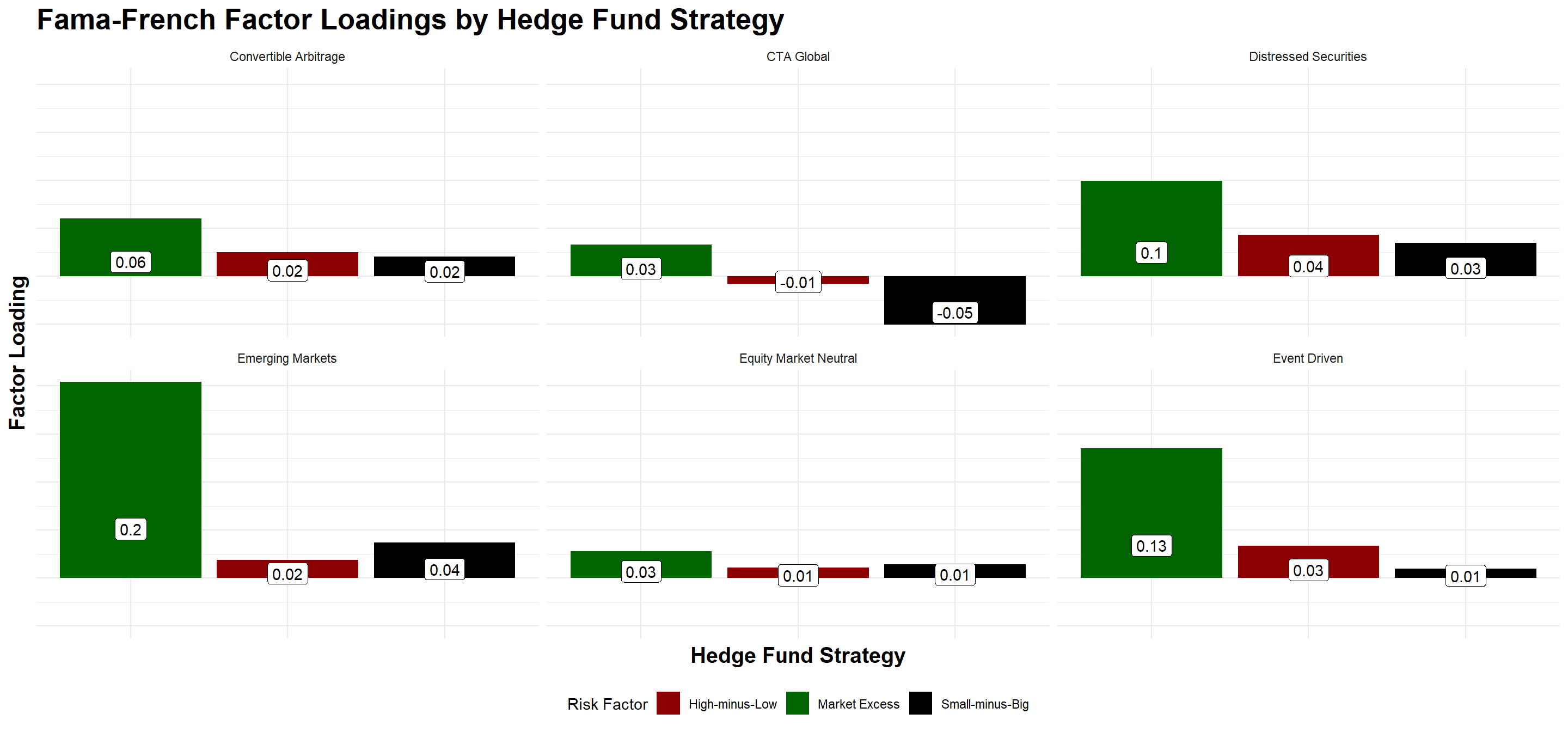

The Performance of Fund Managers

• Some piece of evidence from (Berk and DeMarzo 2023):

  1. The average mutual fund manager can generate value (before computing trading costs and fees, i.e., “gross alpha”)
  2. The median mutual fund manager, on the other hand, destroys value
  3. Only a small portion of managers are skilled enough to add value, according to this reference, in terms of net alpha

• Because individual investors pay fees to fund managers, the net alpha is negative - you should be better-off by putting your money on a passively-managed fund!

• That is, on average, fund managers (“active” strategies) do not provide value after fees, comparing to index funds (“passive strategies”)

The Performance of Fund Managers, continued

If fund managers are high-skilled investors, why they have a hard time adding value?

• One reason why it might be difficult to add value is because there is a trap of liquidity:

  1. If a manager is perceived as skilled, the deposits will grow, making harder to find above-average investment opportunities - that is why you see a lot of closed-end funds
  2. Performance would converge to the mean, at best

• At the end of the day, the market is competitive and people profit following the theoretical predictions

  1. Skilled managers are recompensated for their skills. They capture the economic rents associated with their skills
  2. Investors are not recompensated for the skills of the managers they select - in the end, they derive little benefit, because this superior performance is captured by the manager in the form of fees

Extensions to risk factors - the Factor Zoo

• All in all, what is the gain in performance when using the three-factor Fama-French model relative to the CAPM?

  1. When applied to historical data, results support the three-factor model proposed in (Fama and French 1993)
  2. Fama-French explains over \(\small90\%\) of the diversified portfolios returns, compared with the average \(\small70\%\) given by the CAPM (in-sample performance)

• Importantly, there is a growing number of proposed factors in the Asset Pricing literature - a non-exhaustive list includes:

  1. (Carhart 1997) extend the Fama-French 3-factor model by adding a momentum factor
  2. (Fama and French 2015) extend the Fama-French 3-factor model by incorporating profitability and investment
  3. (Asness, Frazzini, and Pedersen 2013) discuss the role of quality in asset returns

Extensions to risk factors - the Factor Zoo, continued

• All in all, there is a growing number of risk factors that have been documented in the Asset Pricing literature. Such proliferation of risk factors in the literature has been widely known as the “Factor Zoo” (Cochrane 2011)

• Many factors lack theoretical justification or robustness, highlighting the role of replication and out-of-sample validation in factor research:

  1. (Novy-Marx 2013) show that controlling for gross profitability explains most market anomalies and a wide range of seemingly unrelated profitable trading strategies
  2. (Hou, Xue, and Zhang 2015) shows that a model using market, size, investment, and profitability factors argely summarizes the cross section of average stock returns. A comprehensive examination of nearly 80 anomalies reveals that about one-half of the anomalies are insignificant in the broad cross section
  3. (Harvey, Liu, and Zhu 2016) highlight issues with data mining and p-hacking

It is now your turn…

• Using the Hedge Fund monthly returns from the database you have just used to perform the analysis, you will now add two additional factors: Investment and Profitability. The resulting dataset comprises the famous Fama-French Five Factor model. Proceed as follows:

Hands-on Exercise

1. Download the Fama-French 5 Factor portfolios using the download link below (or directly through eClass®)
2. Merge the dataset with the Fama French dataset you have just used. You can use the left_join function to join two dataframes
3. Repeat the procedures we have used before to estimate and chart the output of an OLS regression of the form for all investment strategies:

\[ \small E[R_i] = R_f + \beta_s^M \times \underbrace{(E[R_m]− R_f)}_{\text{Market}} + \beta_s^{SMB} \times \underbrace{E[R_{SMB}]}_{\text{Size}} + \beta_s^{HML} \times \underbrace{E[R_{HML}]}_{\text{Book-to-Market.}} + \beta_s^{RMW} \times \underbrace{E[R_{RMW}]}_{\text{Profitability}} + \beta_s^{CMA} \times \underbrace{E[R_{CMA}]}_{\text{Investment}} \]

How do you interpret your new findings? Does your conclusion hold after including the two additional risk factors?

References

Asness, Clifford S., Andrea Frazzini, and Lasse Heje Pedersen. 2013. “Quality Minus Junk.” AQR Capital Management Working Paper.

Berk, J., and P. DeMarzo. 2023. Corporate Finance, Global Edition. Pearson. https://books.google.com.br/books?id=m78oEAAAQBAJ.

Carhart, Mark M. 1997. “On Persistence in Mutual Fund Performance.” The Journal of Finance 52 (1): 57–82. https://doi.org/10.1111/j.1540-6261.1997.tb03808.x.

Cochrane, John H. 2011. “Presidential Address: Discount Rates.” The Journal of Finance 66 (4): 1047–1108.

Fama, Eugene F., and Kenneth R. French. 1993. “Common Risk Factors in the Returns on Stocks and Bonds.” Journal of Financial Economics 33 (1): 3–56.

———. 2015. “A Five-Factor Asset Pricing Model.” Journal of Financial Economics 116 (1): 1–22.

Harvey, Campbell R., Yan Liu, and Heqing Zhu. 2016“...and the Cross-Section of Expected Returns.” The Review of Financial Studies 29 (1): 5–68.

Hou, Kewei, Chen Xue, and Lu Zhang. 2015. “Digesting Anomalies: An Investment Approach.” The Review of Financial Studies 28 (3): 650–705.

Novy-Marx, Robert. 2013. “The Other Side of Value: The Gross Profitability Premium.” Journal of Financial Economics 108 (1): 1–28.

Scheuch, Christoph, Stefan Voigt, and Patrick Weiss. 2023. Tidy Finance with R. Chapman & Hall/CRC. https://www.tidy-finance.org/r/.

Wickham, Hadley, Mine Cetinkaya-Rundel, and Garrett Grolemund. 2023. R for Data Science. O’Reilly Media. https://r4ds.had.co.nz/.